Exercises — Lesson 9
1. Unstructured Mesh Using "inflation" and "sphere of influence"
Watch the following video for a demonstration on how to create a mesh for the airfoil using the "inflation" and "sphere of influence" features in the Ansys mesher. The advantage of this meshing strategy is that it can be adapted to complex geometries.
2. Verification and Validation of Fluent Results Using a NASA-provided Mesh
Verify and validate the airfoil results from Fluent by comparing with NASA CFD results (verification) and experimental results (validation). Click here for a more detailed description.
3. Angle of Attack Variation
Consider the low-speed airflow over the NACA 0012 airfoil at low angles of attack. The Reynolds number based on the chord is Rec = 2.88 × 10^6. This flow can reasonably be modeled as incompressible and inviscid. Explain why the incompressible, inviscid model for this flow should yield lift coefficient values that match well with experiment but will yield a drag coefficient that is always zero.
Boundary Value Problem
What is the boundary value problem (BVP) you need to solve to obtain the velocity and pressure distributions for this flow at an angle of attack of 10 degrees? Indicate governing equations, domain and boundary conditions (u = 0 at a certain boundary, etc.). For each of the boundary conditions, indicate the corresponding boundary type that you need to select in Fluent.
Coefficient of Pressure
Run a simulation for the NACA 0012 airfoil at angles of attack at 0 degrees and 10 degrees for two cases: a mesh with 15000 elements and a mesh with 40000 elements. Plot the pressure coefficient obtained from Fluent on the same plot as data obtained from experiment. The experimental data from Gregory & O’Reilly, NASA R&M 3726, Jan 1970 can be found with a web search. Follow the aeronautical convention of flipping the vertical axis so that negative Cp values are above and positive Cp values are below. This can be done in MATLAB using set(gca, ’YDir’, ’reverse’);
Lift and Drag Coefficient
Obtain the lift and drag coefficients from the Fluent results on the two meshes. Compare these with experimental or expected values (present this comparison as a table). The experimental values for a 0-degree angle of attack are: Cl = 0.025; Cd = 0.0069, and the experimental values for a 10-degree angle of attack are: Cl = 1.2219; Cd = 0.0138.
Conclusions
Comment on the comparison with experiment for the two angles of attack. Also, comment on the effect of mesh refinement. How does the pressure distribution over the airfoil change on increasing the angle of attack?
4. Multi-Element Airfoil
Consider a three-element airfoil. Download the geometry in STEP format here: 30P30N Airfoil.
The airfoil consists of many points connected by many edges and this STEP file does not have a solid surface. Therefore, to generate the geometry, complete the details of the Import External Geometry as follows:
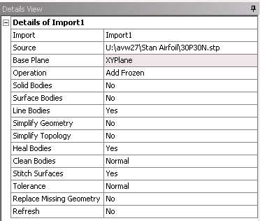
Make sure that Line Bodies is changed from No to Yes. This will ensure that the line bodies of the STEP file are imported into DesignModeler. After this is done, you should have 241 Parts, 241 Bodies in the Geometry Tree.
Now, select the entire 30P30N geometry using Box Select and dragging over the entire geometry.
Select Concept > Surfaces from Edges and click Apply next to Edges to select the edges of the airfoil. After generating the surface, you should have 244 Parts, 244 Bodies in the Geometry Tree. You can go into the Geometry Tree and select all edges of the 30P30N airfoil and create a part from them and suppress the line bodies in the part.
In the XY Plane, create a new sketch. This will be the start of the flow domain and is similar to the creation of the flow domain in this tutorial. Dimension the arc to have a radius of 3.5 m and the rectangle section to have a horizontal distance of 7 m behind the airfoil. After generating this surface, follow the same procedure outlined in this tutorial to subtract the multi-element airfoil surface body from the flow domain surface body. Close DesignModeler and open Meshing.
You should have only the surface body in the tree under geometry. Because of the way the geometry was created, there are many edges that create the airfoil. For convenience, a virtual body will be created on each element for the creation of the mesh.
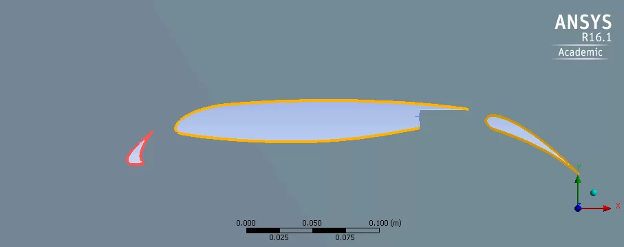
Select Model in the outline tree and in the toolbar, click on Virtual Topology. Using Box Select, drag the cursor over the first element and select all edges. Right Click and select Insert > Virtual Cell. Repeat this for the remaining elements. You should see something similar to the image below.
For the second element, the right angle at the trailing edge should be independent edges and do not need to be included in the virtual cell selections. This will come in handy for the inflation layers in the mesh generation.
Now the edges have been merged for each airfoil element and edges can be selected independently.
The mesh generation is similar for this geometry as it is for the single-element airfoil. Differences arise when generating the inflation layer due to the small gaps between elements. Make sure the advanced sizing function is on for curvature. Each edge will need to be sized and an inflation layer generated on each edge.
Once the mesh is properly generated, create the named selections. This process is identical to the airfoil case outlined in this tutorial with all elements of this airfoil being designated as "airfoil" under named selections.
Open Fluent and change the model to realizable k-e. The boundary conditions are the same as for the airfoil in this tutorial.
You are being redirected to our marketplace website to provide you an optimal buying experience. Please refer to our FAQ page for more details. Click the button below to proceed further.