Pre-Analysis & Start-Up — Lesson 2
Ansys Student software can be downloaded for free here.
In the Pre-Analysis step, we will review the following:
- Assumptions: Assumptions for classical Hertz contact mechanics are discussed.
- Mathematical model: Governing equations and boundary conditions, as well as additional relations will be discussed.
- FEM approach: We will discuss the solution strategy used in solving a nonlinear problem in FEM.
Assumptions
This problem is a classic example of Hertz Contact Mechanics*, and hence, makes the following assumptions:
- Surfaces are continuous and non-conforming, which means that initial contact is a point or a line. In our example of sphere-plate, the initial contact interface is in a form of a point.
- Strains are small.
- Solids are elastic. This means that the material response of stress and strain behaves linearly.
- Surfaces are frictionless and cannot penetrate into each other.
For analytical solution, the following additional assumption is made;
- Both objects (in our case, sphere and plate) are semi-infinitely large bodies (R1,R2 >> a, where a is contact radius).
Reference* S. Timoshenko and J.N. Goodier: “Theory of Elasticity,” Chap. 13: Sect. 125, “Pressure between Two Spherical Bodies in Contact"
Mathematical Model
As in any static analysis, the fundamental governing equations that we must keep in mind are the stress equilibrium equations (i.e., governing equations).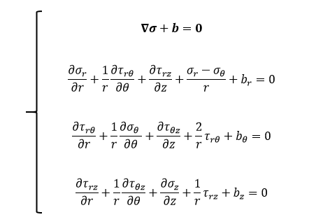
In the above set of equations, it can be shown that σij = σji due to moment balance! Furthermore, we begin by making valid assumptions with regards to our problem of interest. First, we assume that there is no body force (b = 0) anywhere in our model. In addition, we model our problem as a plane stress problem, which means that all of the out-of-plane stress components involving θ-direction can be assumed to equal zero (σθ = τθr = τθz = 0). These assumptions lead to the following simplifications: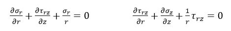

Next, we list the relevant boundary conditions of our problem. The two types of boundary conditions, essential and natural, will be specified for all boundaries in our model. It must be noted that essential boundary conditions refer to displacement conditions and natural boundary conditions represent traction conditions. It is also important to observe that only one of these boundary conditions may be specified at a given boundary. In addition, only one of these boundary conditions is sufficient for a given boundary point.
Along the frictionless contact interface, we specify the following boundary conditions.![]()
Here, r represents the radial position away from the axis of symmetry and a denotes the contact radius. We note that, due to the nonlinear nature of our problem, the contact radius a will change throughout the loading process. Even though the contact interface between the sphere and the surface is initially a single point, the contact interface will grow to become a surface as the sphere deforms.
Since the top of sphere is subjected to a point load, a traction condition is specified at this location. We observe that since the load is being applied to a point, traction will be infinitely large.![]()
Along the free surface of the sphere, the boundary condition may be specified as follows.![]()
With symmetry condition, the following boundary condition is prescribed along the axis of symmetry.![]()
By identifying the governing equations and defining the boundary conditions, we have set up the mathematical model. We will now establish several additional relationships, which are used in the postprocessing step for computing stress and strain fields using these nodal displacements. These relationships are commonly referred to as the constitutive equations. One of these equations is the strain-displacement relationship.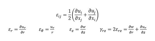
The second relationship is called Hooke’s law. For our model, we assume an isotropic material under plane stress, and so further simplifying the Hooke’s law results in the following equations: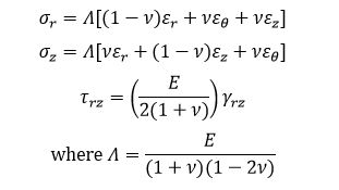
FEM Approach
In this section, we discuss the general methods that Ansys software uses in solving for the desired results. As the name suggests, the finite element method first requires meshing the system that is to be analyzed into a finite number of elements. In Ansys simulations, one can manually create the mesh configuration, or can alternatively let the software use a special algorithm to generate the mesh profile, which will not be discussed in this tutorial. Depending on the level of accuracy of the results that is desirable, one can choose to refine the mesh, so that there will be more elements near any region in the model. Having a greater number of elements in the system can allow the results to converge within appropriate bounds. It should also be noted that an element is generally comprised of multiple nodes. Configuration of the nodes in each element can vary for different element types. As an example, an element, PLANE183, has the configuration, as shown below.
Each of the eight nodes shown above can be described by displacement vectors (translational and rotational components, depending on the element type) and by force vectors. The finite element method first solves for the nodal displacement field with the specified boundary conditions. The underlying system of equations that Ansys solves for is shown below.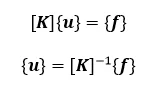
Here, [K] is also referred to as the global stiffness matrix, and contains n by n components, where n is equal to the total degrees of freedom of the system. On the other hand, {u} and {f} are column matrices with n components, which represent nodal displacement fields and nodal force fields, respectively. After specifying the appropriate boundary condition in Ansys, it then solves for these displacement and force fields simultaneously.
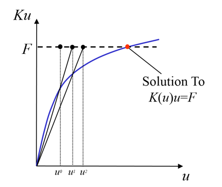
However, in the case of our Hertz contact example, we note that the system is a highly nonlinear problem, due to the mechanical interactions between multiple components of the system. The fact that the boundary condition at the contact interface between the sphere and the rigid plate changes throughout the loading process indicates that an iterative approach is necessary to converge the solutions. More specifically, we observe that the state of traction and the stiffness of the system depend on the displacement near the contact interface.![]()
By default, Ansys requires that force reaction balance be satisfied within a given tolerance level. If the method of linear analysis is selected, solution would most likely fail to converge for a system that contains a variable contact interface since only a single iteration would be performed. To overcome this issue, we introduce the Newton-Raphson (NR) method in solving for the solution. Given an initial guess, the NR method generates a sequence of guesses that converges to a root of the equation. This method is based on making successive approximations to solution using the previous value of u to determine K(u).![]()
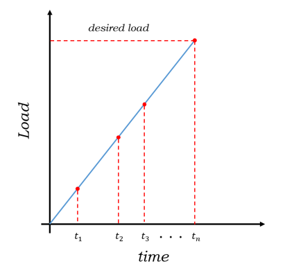
In addition to the Newton-Raphson method, other techniques can be applied, to help fix convergence issues that might arise. This method, known as Incremental Loading technique, subdivides the load into smaller steps. While increasing the number of substeps may require more computation, it helps to linearize the solution by making smaller loads, such that the residuals between iterative solution and true solution also become smaller. It must be noted that these two techniques can be applied to our finite element analysis individually or can be used simultaneously. Using both of these, however, is highly recommended, since the Incremental Loading technique can help decrease the number of iterations required to obtain a converged solution.
Once the solution has converged, the nodal displacement fields obtained from the final equilibrium iteration can be further used to generate the strain and stress distribution at each node. In FEM, analyses, similar to the ones found under Mathematical Model section, are adopted to compute these nodal fields. However, we have to modify our approach slightly to take into account the fact that we now have a finite number of elements. This calls for a linear, first-order approximation method among the neighboring elements in computing strain distribution. In other words, the nodal strain and stress fields are calculated in the following manner: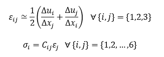
Start-Up
The following video shows how to create a project and set up engineering data for our problem.
You are being redirected to our marketplace website to provide you an optimal buying experience. Please refer to our FAQ page for more details. Click the button below to proceed further.